This is a notebook, not a finished essay. I’m learning quantum computing from first principles and writing up each part as I go. My two main texts are Thomas Wong’s Introduction to Classical and Quantum Computing and Nielsen and Chuang’s Quantum Computation and Quantum Information.
1. Why?
I wrote an article exploring artificial intelligence and quantum computing as breakthrough technologies. As a software engineer at the time, I was curious about what they were, how they worked, and the problems they could solve.
I pursued a master's degree in artificial intelligence. Since then, my work has evolved into research with interests in ML interpretability.
Quantum machine learning is where those threads meet: models whose internal states can't be observed without disturbing them make interpretability both harder and more important. I now lead the quantum ML subfield at Cohere Labs Open Science Community, and we are building an open-source platform to make the fundamentals accessible to beginners.
In many ways, this feels like a full-circle moment: returning to a question that first captured my curiosity in 2020, now equipped with the experience to investigate it more deeply.
Interested in joining the quantum ML group? →Why start with classical computing?
People sometimes say we’re in the vacuum tube era of quantum computing. Classical computers went through the same stage:
Alan Turing describes the Turing machine, the founding model of computation.
Shockley, Bardeen and Brattain build the transistor at Bell Labs.
Tom Kilburn runs the first stored program, ending the era of rewiring vacuum tubes by hand.
Computers in the 1940s were room-sized machines built from thousands of parts that could fail. Today we rarely think about the billions of transistors in a laptop. Quantum computers are still at the early stage: researchers are working out how to build large, reliable computations from noisy physical qubits. Classical computing already answered many of the same engineering questions, so it’s the natural place to start.
A bit is an abstract unit of information; a transistor is one physical device that stores it. Likewise, a qubit is an abstract unit of quantum information that can be built from superconducting circuits, trapped ions, neutral atoms or photons. This notebook is about the abstractions.
2. Mathematical foundations
Bits and states
A coin has two states, heads or tails. Two coins have four (HH, HT, TH, TT), and coins have . Any two-state system (a coin, a switch, a transistor) can be labelled 0 and 1, a bit: the smallest unit of classical information. Everything else, numbers in binary and text in ASCII or Unicode, is built from strings of bits.
The key fact: bits can be in any one of states, but only one at a time.
A general pure state of qubits is described by complex amplitudes, one for each classical bit string. That exponential growth is why simulating a generic quantum state gets hard as qubits are added. But a large state space is not, by itself, a quantum advantage: an algorithm still has to use operations and interference to extract useful information, and the interesting question is whether it can solve a particular problem faster than the best classical method.
Logic gates and universality
Gates transform bits, and a truth table fully describes a gate:
| AND () | OR () | XOR () | NAND () | ||
|---|---|---|---|---|---|
| 0 | 0 | 0 | 0 | 0 | 1 |
| 0 | 1 | 0 | 1 | 1 | 1 |
| 1 | 0 | 0 | 1 | 1 | 1 |
| 1 | 1 | 1 | 1 | 0 | 0 |
There are 16 possible two-bit gates and 256 three-bit gates, but we don’t need them all. A universal gate set can build any truth table. {NOT, AND, OR} is universal, and so is NAND alone: tie its inputs together to get NOT (), and NOT a NAND to get AND. Gates combine into circuits. Built from AND, OR and XOR gates, a full adder takes 5 gates, so a ripple-carry adder for two -bit numbers takes ; more generally, addition needs elementary operations. Boolean algebra (such as De Morgan’s law ) shrinks circuits further.
Quantum computing has universal gate sets too, such as {H, T, CNOT}: circuits built from them can approximate any unitary operation to arbitrary accuracy. That’s what makes quantum circuits programmable. (General quantum operations also include measurement and noise, which aren’t unitary and need a broader description.)
Whiteboard notes: adders and Boolean algebra
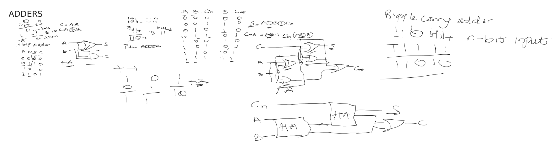
Half adder (, ), full adder from two half adders, ripple-carry addition.
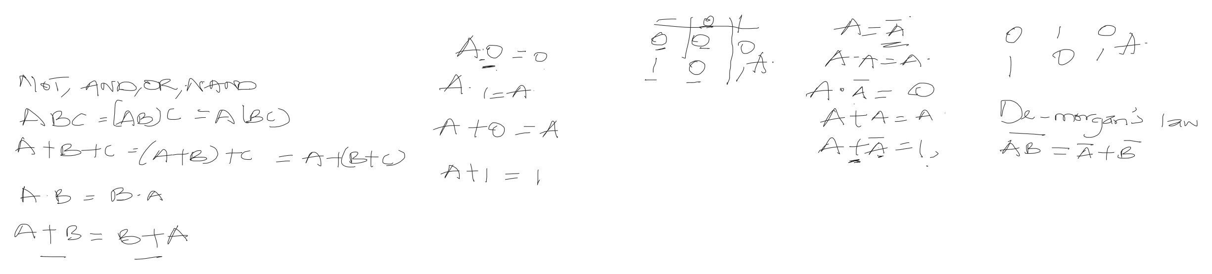
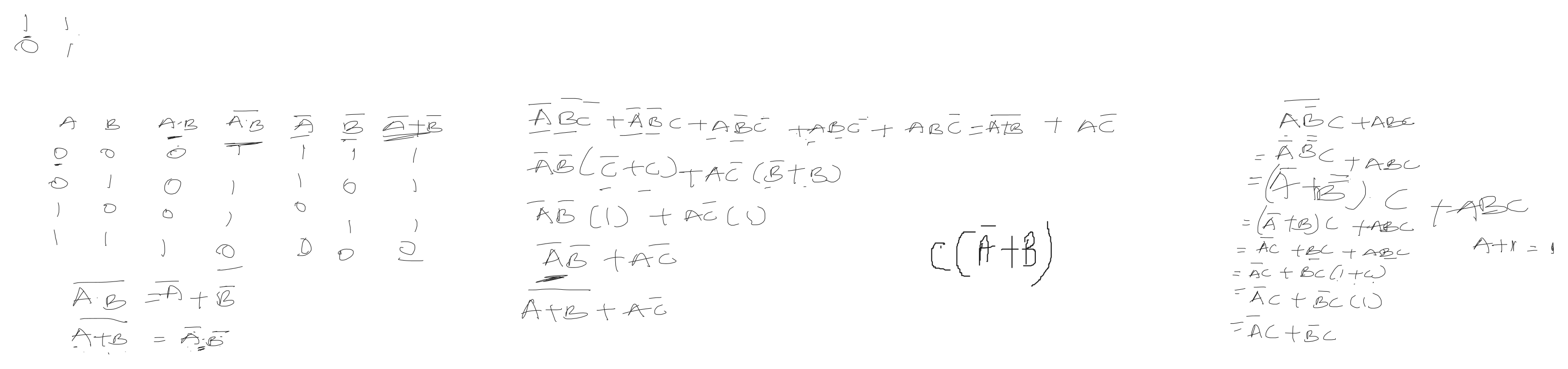
Proving De Morgan’s law, and simplifying to .
Reversible gates
A gate is reversible if its output always tells you its input. That needs as many outputs as inputs, and no output repeated. NOT is reversible. AND isn’t: an output of 0 could have come from 00, 01 or 10, so information is lost.
The Toffoli gate fixes this. It keeps its inputs and XORs the AND into a third bit: . With it computes AND, with it computes NAND, so (with extra ancilla bits) it’s universal for classical reversible computation. It flips only when , hence its other name, controlled-controlled-NOT. The same trick makes any function reversible: .
Whiteboard notes: reversible gates and the Toffoli gate
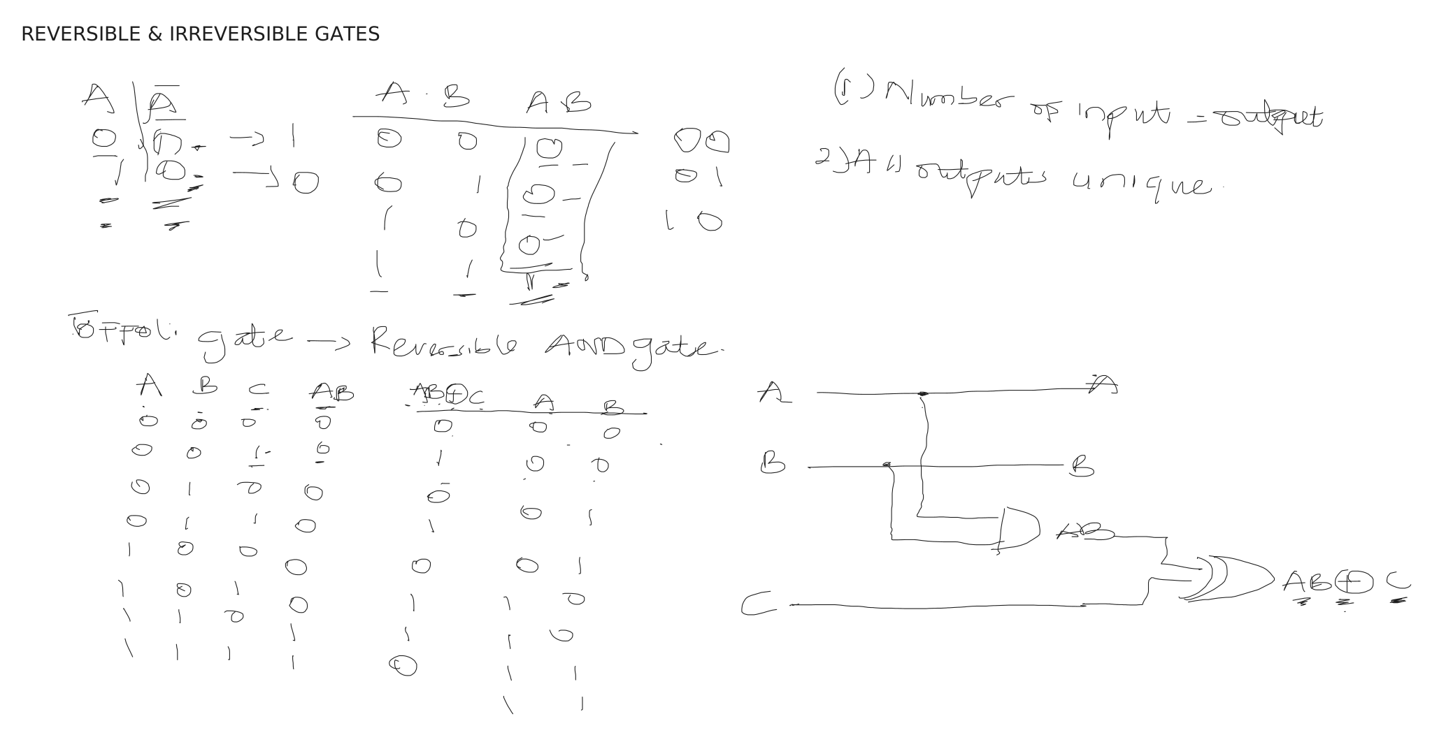
Ideal quantum gates are unitary, and every unitary is reversible, so this isn’t optional. Not every physical operation is: measurement and noise are irreversible. The Toffoli gate is itself a quantum gate, and the construction is exactly how quantum algorithms like Grover’s and Shor’s query a classical function, as an oracle.
Error correction
Bits flip by accident. In a 2003 Belgian election, one candidate gained exactly votes, suspected to be a cosmic-ray particle flipping a single bit. The fix is redundancy: encode one logical bit in several physical bits.
With the three-bit repetition code, and , and a single flip is corrected by majority vote. Better still, two parity checks (, ) pinpoint which bit flipped without revealing the encoded value. The code fails only if two or three bits flip, with probability , which beats an unprotected bit whenever .
Whiteboard notes: repetition codes and parity checks
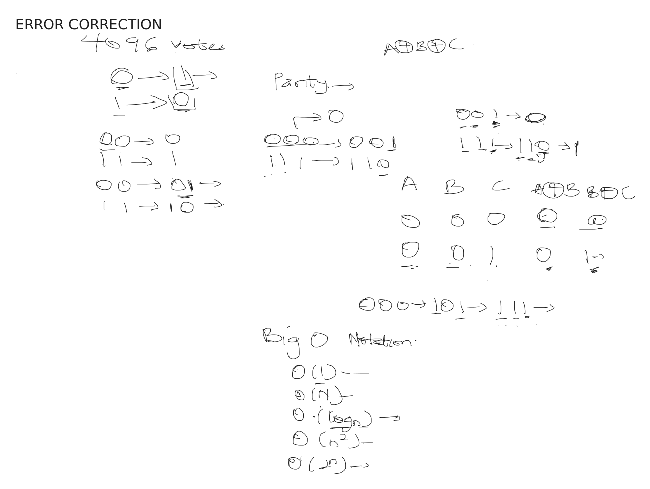
Qubits are far noisier than transistors, and two new constraints appear: an unknown quantum state can’t in general be copied perfectly (the no-cloning theorem), and measuring it can disturb it. Quantum error correction is built on the same idea as the parity checks here: extract information about which error happened without revealing the encoded logical state.
Complexity: what’s possible, and what’s efficient
Algorithms are compared by how their cost grows with input size , using Big-O notation: and are polynomial and usually tractable, while is exponential and quickly isn’t.
Some problems can’t be solved at all. Turing proved the halting problem (will this program ever stop?) is undecidable: any supposed solver can be fed a program built to do the opposite of whatever predicts about it.
Solvable problems are grouped into complexity classes. A class describes the resources needed to solve a whole family of problems as the input grows, not a category of individual algorithms:
- P: solvable in polynomial time.
- NP: answers can be checked in polynomial time. Whether P = NP is a million-dollar open problem.
- BPP: solvable in polynomial time with randomness and a small error probability.
- BQP: solvable in polynomial time by a quantum computer.
None of these inclusions is known to be strict, and there’s no known efficient quantum algorithm for NP-complete problems.
Quantum computers can’t solve undecidable problems. What they may do is make some hard problems tractable. Shor’s algorithm factors integers in polynomial time on a sufficiently large, fault-tolerant quantum computer; that’s a theoretical result, and today’s machines can’t break practical RSA keys. Grover’s algorithm solves unstructured search with oracle queries, versus classical queries in the worst case. That challenges the strong Church–Turing thesis, the idea that a probabilistic classical computer can efficiently simulate any reasonable model of computation.
The thread, in one table
| Classical | Quantum |
|---|---|
| Bit: 0 or 1 | Qubit: a superposition of and |
| bits: one of states | qubits: amplitudes (pure state) |
| Logic gates, universal set {NAND} | Quantum gates; {H, T, CNOT} approximates any unitary |
| Reversible computing is optional (Toffoli) | Ideal (unitary) gates are reversible; Toffoli is one too |
| trick | Quantum oracles in Grover’s and Shor’s algorithms |
| Repetition code, parity checks | Quantum codes, syndrome measurement without reading data |
| Read a bit any time | Measurement gives one outcome and can disturb the state |
| BPP | BQP |
3. From classical bits to quantum bits
Superposition, informally
Meet Schrödinger’s cat, a thought experiment by Erwin Schrödinger. Put a healthy, sleepy cat in a box with a radioactive atom that may or may not decay by the end of the experiment. The atom can’t hurt the cat, but if it decays it triggers a Geiger counter wired to an alarm clock that rudely wakes the cat.
The thought experiment asks what happens when a microscopic quantum event is linked to a macroscopic outcome. It’s often summarised as “the cat is both asleep and awake until someone looks”, which is memorable but misleading. Schrödinger meant it to show the tension between quantum mechanics and our everyday intuition about large objects, not to describe what quantum theory literally says about cats.
It helps to separate three ideas that are easy to blur together:
- Classical uncertainty: the system is in one definite state; you just don’t know which. A coin under a cup is like this.
- Quantum superposition: the state is a combination of basis states with amplitudes, and those amplitudes can interfere. That’s not a statement about our ignorance, and an isolated system can stay in superposition while it evolves.
- Decoherence: interactions with the environment make interference between the alternatives effectively impossible to observe.
Measurement produces an outcome with probabilities set by the quantum state and by which measurement is performed. Measuring can disturb the state, but it doesn’t wipe out every superposition: what happens depends on what you measure. How definite outcomes arise from quantum evolution is still a foundational question, and it’s part of why Schrödinger and Einstein found the theory so uncomfortable.
The double-slit experiment makes interference concrete. Fire electrons one at a time at a barrier with two narrow slits. Each electron arrives at the screen as a single dot. But after many electrons, the dots build up an interference pattern: the amplitudes for the two paths combine, adding in some places and cancelling in others. If the setup makes which-path information available, through any measurement or interaction that records the slit, not a person watching, the pattern disappears and you get two bands. When the paths stay coherent and indistinguishable, they interfere.
This is also the first glimpse of a theme that runs through the rest of the notebook: a single measurement gives one outcome, and the quantum state shows up in the statistics of many repeated measurements.
Why does superposition help computation?
This was the big question I had after reading about superposition. Imagine searching for one specific cat among 1,000.
A classical computer checks cats one by one, and in the worst case checks all 1,000.
A quantum computer can prepare a superposition that includes all 1,000 candidates at once. But it can’t just look at all of them and report the right one. Measuring immediately gives one random candidate, which is probably wrong.
The secret is interference. Each candidate carries an amplitude, a number related to its probability of being measured. Unlike probabilities, amplitudes can be negative (or complex), so they can cancel out, like waves.
- Prepare a superposition where every candidate has the same amplitude, so all are equally likely.
- Interfere. Apply carefully designed operations that mark the target (in Grover’s algorithm, by flipping the sign of its amplitude) and then make amplitudes interfere so the target’s grows and the others shrink. Repeat.
- Measure. The target is now very likely to come out.
It’s a bit like tuning a radio: you’re not listening to every station separately, you’re shaping the signal so the one you want comes through clearly. It’s not a perfect analogy, but it gives the intuition.
Superposition lets the quantum state hold amplitudes for many possible answers. Interference makes some answers more likely and others less. Measurement gives a classical answer, ideally a useful one. Superposition alone gives no advantage; it gives the algorithm amplitudes to work with, and interference is how the algorithm shapes which outcome the measurement is likely to give.
Qubits
A qubit is like a classical bit in one way: it has two basis states, 0 and 1. In Dirac or bra-ket notation, we write them as kets:
We can picture them as the north and south poles of a sphere of radius 1, the Bloch sphere. Following the physics convention, the -axis points out of the page, the -axis points to the side and the -axis points up. Then sits at and at .
A classical bit can only be at one pole or the other. A qubit can be in a superposition of and , for example equal parts of each:
Both coefficients are , so this state is halfway between the poles, on the equator. It sits where the Bloch sphere meets the -axis, at .
Every point on the equator is equal parts and . What distinguishes them is the relative phase between the two terms. A phase of moves the state to the -axis, and the complex phases and move it to the -axis. This is the first place complex numbers show up in quantum computing.
| State | Definition | Bloch point | Prepared from by |
|---|---|---|---|
| H | |||
| H, then Z | |||
| H, then S | |||
| H, then S† |
In Qiskit, each state is a one-qubit circuit (which starts in ) followed by a couple of gates. For example, :
from qiskit import QuantumCircuit
from qiskit.quantum_info import Statevector
from qiskit.visualization import plot_bloch_multivector

qc = QuantumCircuit(1)  # one qubit, initialised to |0>
qc.h(0)                 # Hadamard: |0> -> |+>, onto the equator
qc.s(0)                 # S: phase of +i on |1>, rotates |+> to |i>
state = Statevector.from_instruction(qc)

plot_bloch_multivector(state)
Swapping s for z gives , sdg gives , and an x gate on its own gives :
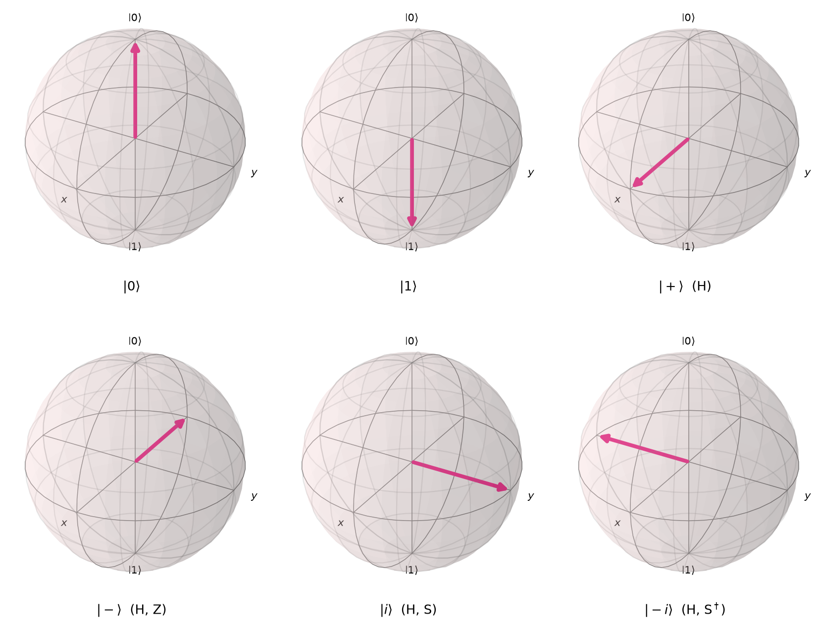
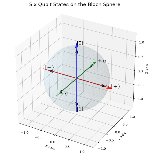
The full notebook from the cohort session, with exercises on gate identities like , and , is on Colab.
These four are just the points where the axes cross the equator. Other complex phases reach every other point on the equator, and superpositions aren’t limited to the equator either. A qubit can be at any point on the Bloch sphere. That continuous space of states, together with interference, is what the rest of this notebook builds on.
Coming next
Planned
The title promises a path to interpretability, and this first entry only gets as far as a single qubit. Here’s the plan for the next entries:
Born's rule, measuring in different bases, and why a single shot gives one outcome while the state only shows up in the statistics of many.
Tensor products, where the 2n amplitudes come from, and multi-qubit gates such as CNOT and Toffoli.
States that can't be described qubit by qubit, Bell states, and what entanglement does and doesn't let you do.
Quantum systems can be measured and studied, but access to their states is constrained and fully characterising a general state is expensive. What does it mean to interpret a quantum machine learning model under those constraints, and which tools from classical ML interpretability carry over?
Main texts: Thomas G. Wong, Introduction to Classical and Quantum Computing, Rooted Grove, 2022 (free PDF from the author); Michael A. Nielsen and Isaac L. Chuang, Quantum Computation and Quantum Information, 10th anniversary edition, Cambridge University Press, 2010. Cohort notebook: Chapter 2, part 1 on Colab.